Irene
From ancient Greek, Εἰρήνη, meaning peace.
The S1 and S2 signals are localized to relatively short time intervals within the sensors’ waveforms. Thus, Irene processes RWFs coming from either the Decoder (detector) or from Diomira (MC). The city finds these time slices (peaks) and disregards the rest of the waveform. During this procedure, PMT and SiPM waveforms are matched and combined into a single structure. The collection of all peaks in an event is called a Peak-map or PMap.
Input
/Run/events
/Run/runInfo
/RD/pmtrd
/RD/sipmrd
Output
/PMAPS/S1: the sliced PMT-summed waveform for each S1 peak. 4 columns: event number, peak number, time (\(\mu\)s) and amplitude (pes)
/PMAPS/S1Pmt: the sliced individual PMT waveforms for each S1 peak. 4 columns: event number, peak number, pmt index (npmt) [1] and amplitude (pes)
/PMAPS/S2: the sliced PMT-summed waveform for each S2 peak. 4 columns: event number, peak number, time (\(\mu\)s) and amplitude (pes)
/PMAPS/S2Pmt: the sliced individual PMT waveforms for each S2 peak. 4 columns: event number, peak number, pmt index (npmt) [1] and amplitude (pes)
/PMAPS/S2Si: the sliced individual SiPM waveforms for each S2 peak. 4 columns: event number, peak number, sipm index (nsipm) [1] and amplitude (pes)
/Filters/empty_pmap: flag for whether an event passed the empty pmap filter
/Filters/s12_indices: flag for whether an event passed the s12 indices filter
Config
Besides the Common arguments to every city, Irene has the following arguments:
Parameter |
Type |
Description |
|---|---|---|
|
|
Number of waveform samples to compute the baseline. |
|
|
Number of waveform samples to compute the MAW. |
|
|
Threshold for MAW calculation in \(pes\). |
|
|
Threshold for individual SiPM samples. Can be absolute (\(pes\)) or relative (unitless), depending on |
|
|
Thresholding mode for individual SiPM samples. |
|
|
Lower/upper limits to the width of S1/S2 signals expressed in number of samples. |
|
|
Lower/upper limits of the search window for S1/S2 signals. |
|
|
Rebin factor for S1/S2 signals. Rarely changed. 1 for S1 and 40 for S2 signals. |
|
|
Allowed range of signal fluctuations below threshold for peak merging expressed in number of samples. |
|
|
Threshold applied to the PMT-summed waveform in order to find S1/S2 peaks. |
|
|
Threshold applied to the time-integrated signal of each SiPM to discard SiPMs with only dark counts. |
|
|
Sampling period of PMTs. Should be removed. |
|
|
Sampling period of SiPMs. Should be removed. |
Workflow
Irene performs a number of data transformations in order to obtain a PMap. These operations can be grouped in four main tasks, performed in the following order:
Deconvolution of PMT waveforms
Due to the bias configuration of the PMTs, the PMT waveform does not represent the actual signal produced by the PMT, but its derivative (for details see [2]). The typical PMT RWF for a Kr event looks like this:
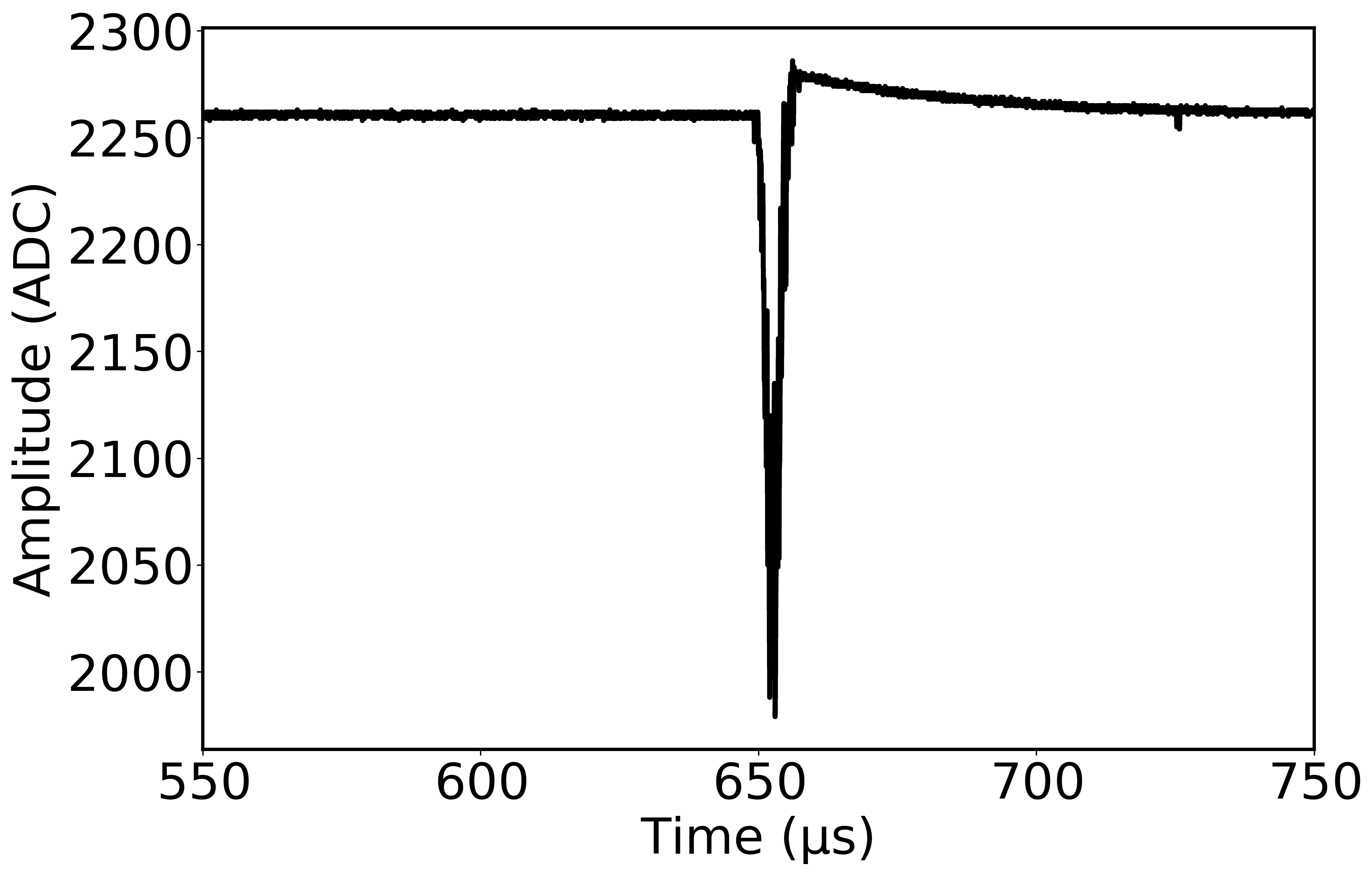
This waveform needs to be transformed into a unipolar (positive-defined) zero-baseline waveform whose area is proportional to the number of photons detected. The part of the waveform corresponding to when the PMT doesn’t receive any light is just a gaussianly-distributed noise around a baseline value. This value is estimated using the first few microseconds of the waveform; the amplitude is averaged over this time frame and subtracted from the entire waveform to produce a baseline-subtracted waveform.
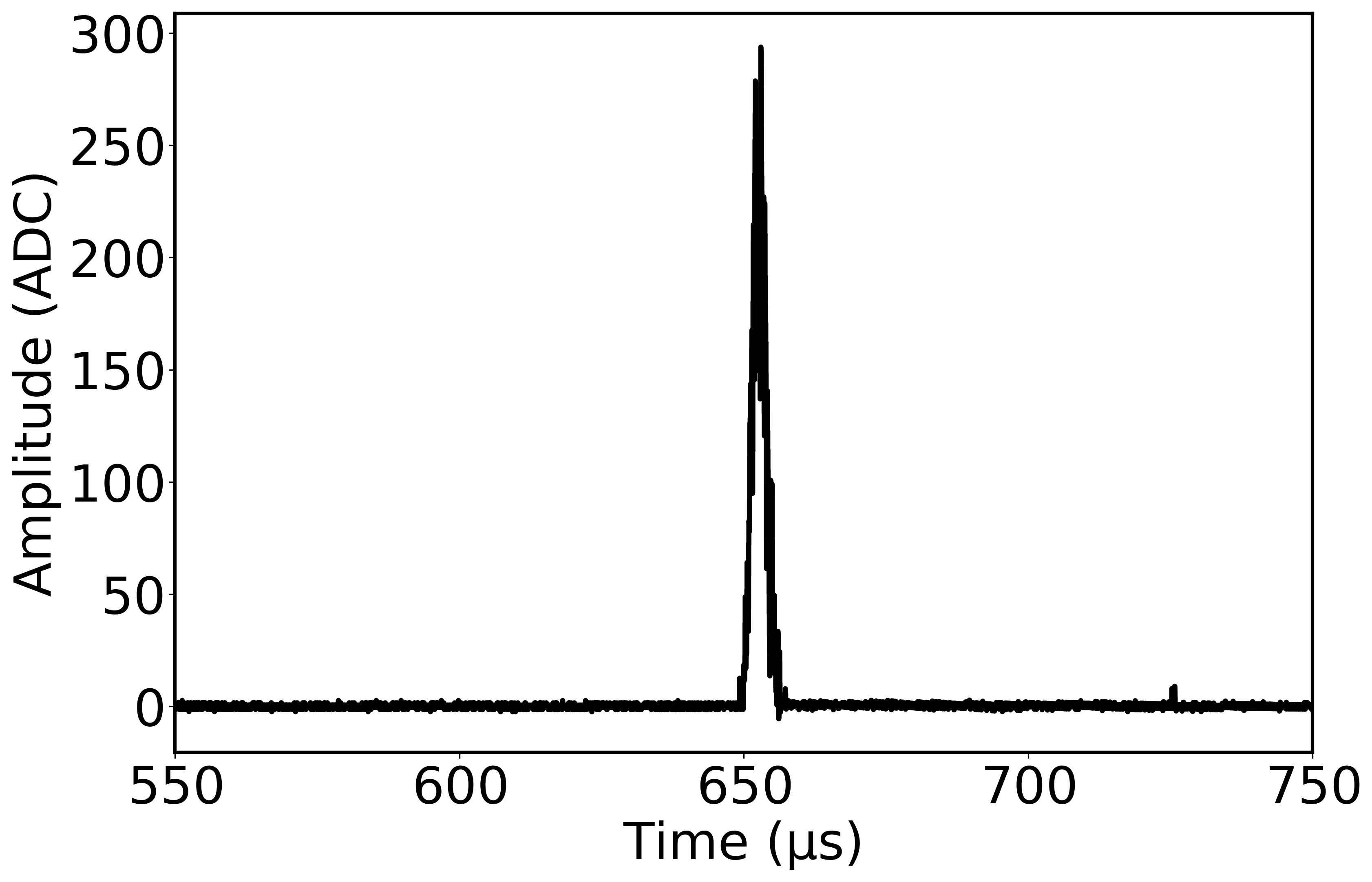
The resulting waveform is still bipolar. This is addressed by the deconvolution algorithm (BLR). This process is fairly complex, but in simple terms, it consists of a high-pass filter and a signal accumulator, which inverts the effect of the PMT electronics. For greater detail on the PMT electronics and the recovery algorithm see [2]. Finally, the polarity of the waveform is inverted to make it positive.
All the aforementioned steps are performed for each PMT separately. The output of this algorithm are the so-called Corrected waveforms (CWFs).
The city Isidora allows the user to run just this stage of the reconstruction and store the CWFs for further study. Irene however, does not store them and they are fed directly into the rest of the PMap-building algorithm. The CWF corresponding to the RWF shown above is:
Baseline subtraction of SiPM waveforms
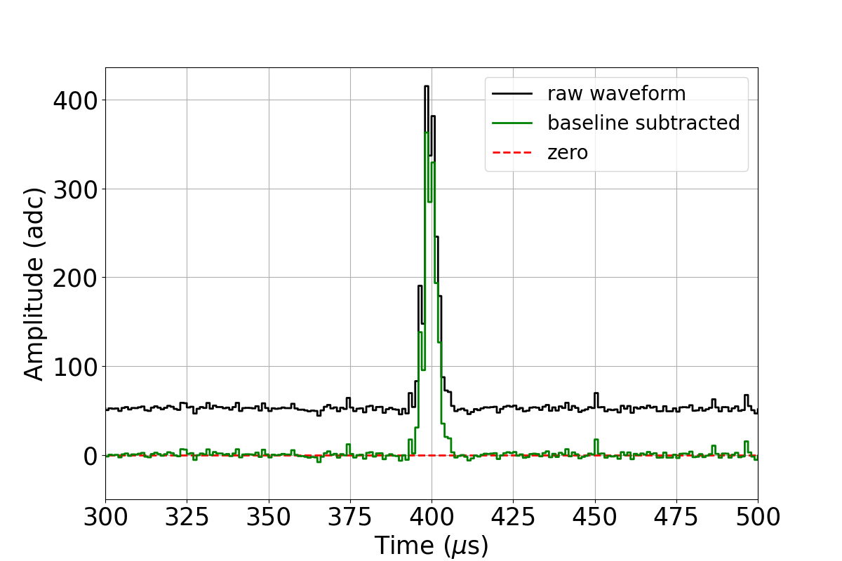
Unlike PMTs, SiPM waveforms are already unipolar and positive-defined. The baseline computation for SiPMs is slightly different. Instead of averaging a fraction of the waveform, the mode [3] of the entire waveform is used. The baseline is estimated and substracted on an event-by-event basis and for each SiPM independently. The following figure shows a comparison between a SiPM RWF and a baseline-subtracted SiPM waveform.
Waveform calibration
The production and manufacturing of the sensors and other electronic components does not guarantee a homogeneous response among all sensors. Thus, the waveforms are calibrated to equalize their response. The calibration consists of a constant for each sensor indicating the number of ADC corresponding to a photoelectron (calibration constant), which is a physical quantity common to all of them. The calibration technique is similar for PMTs and SiPMs. For details about the calibration procedure see the calibration cities: Berenice, Phyllis and Trude.
The calibration constants are measured regularly while the detector is in operation. The calibration constants are fetched from the database automatically and indexed by run number.
The calibration step is rather simple. The CWF of each PMT and the baseline-subtracted waveform of each SiPM are scaled up according to their corresponding calibration constants. The resulting set of waveforms are sometimes called CCWFs (Calibrated Corrected Waveforms).
Peak finding and matching of PMT and SiPM signals
The peak finding and waveform slicing is arguably the most complex part of the RWF processing. The algorithm must be able to find two very different types of signals (S1 and S2), while accurately establishing the limits on those peaks to maintain the energy resolution capabilities of the detector.
In order to optimize the peak search, PMT CCWFs are used as they have a higher sampling rate and therefore better time resolution. The searches for S1 and S2 signals use slightly different waveforms. The PMT waveforms contain some low-frequency noise that can shift the PMT baseline locally by a small amount. The MAW (Moving Average Window) accounts for these small local variations of the baseline, allowing for a higher peak finding efficiency. The parameter n_maw controls the size of this window. The S1 peak search is performed by looking for samples of the PMT waveform that deviate from the MAW-generated baseline more than thr_maw. On the other hand, the S2 peak search uses the CCWFs directly, without a MAW.
On top of that, these waveforms are PMT-summed to increase the signal-over-noise ratio [4]. For S1 peaks, this summation is only applied for samples above thr_maw. S1 and S2 signals are searched independently.
The PMT-summed waveform is searched for samples above a certain threshold (thr_csum_sX), which may depend on the event type. The samples below the threshold are initially ignored. However, fluctuations in the PMT signal close to the threshold can lead to a split in an otherwise continuous peak. This is particularly relevant for S1 signals due to their small amplitude in low-energy events.
To minimize this effect, signal regions separated by a short time (configurable via the sX_stride arguments) are joined back together. This stride may also depend on the event type.
In order to reduce the amount of spurious or unphysical peaks, the search can be restricted to certain time spans (sX_tmin, sX_tmax) in the waveform.
Furthermore, the resulting peaks are filtered based on their width (via sX_lmin, sX_lmax), improving the efficiency of finding peaks corresponding to a true signal.
The beginning and end of the signal region is kept for each peak. This information is then used to slice each PMT and SiPM waveforms.
To create a S2 peak, the sliced PMT waveforms are resampled according to s2_rebin_stride. By default, this resamples from 40 MHz (25 ns) to 1 MHz (1 \(\mu\)s) to match the sampling rate of SiPMs. Also, SiPMs are noisier than PMTs, producing spurious photoelectron pulses. In order to minimize this effect, a threshold thr_sipm is applied to each sample of each SiPM, suppressing values below it. This threshold can be common to all SiPMs, or applied to each individual SiPM, based on their measured noise spectrum. This behaviour can be controlled via the thr_sipm_type argument. Finally, due to the characteristics of the tracking plane, most SiPMs don’t contain signal. Hence, another threshold the_sipm_s2 is applied to the time-integrated signal of each SiPM for a given peak [5].
The resulting PMT and SiPM waveforms are then time-matched and stored in a single object (Peak).
S1 signals on the other hand, are weak enough to be detected only by PMTs, therefore the SiPMs are ignored during the S1 search. The waveforms can also be resampled using the s1_rebin_stride, however this parameter is usually set to 1 to keep the optimal time resolution of S1 signals.
The following figure shows the performance of this algorithm on a typical Kr event.
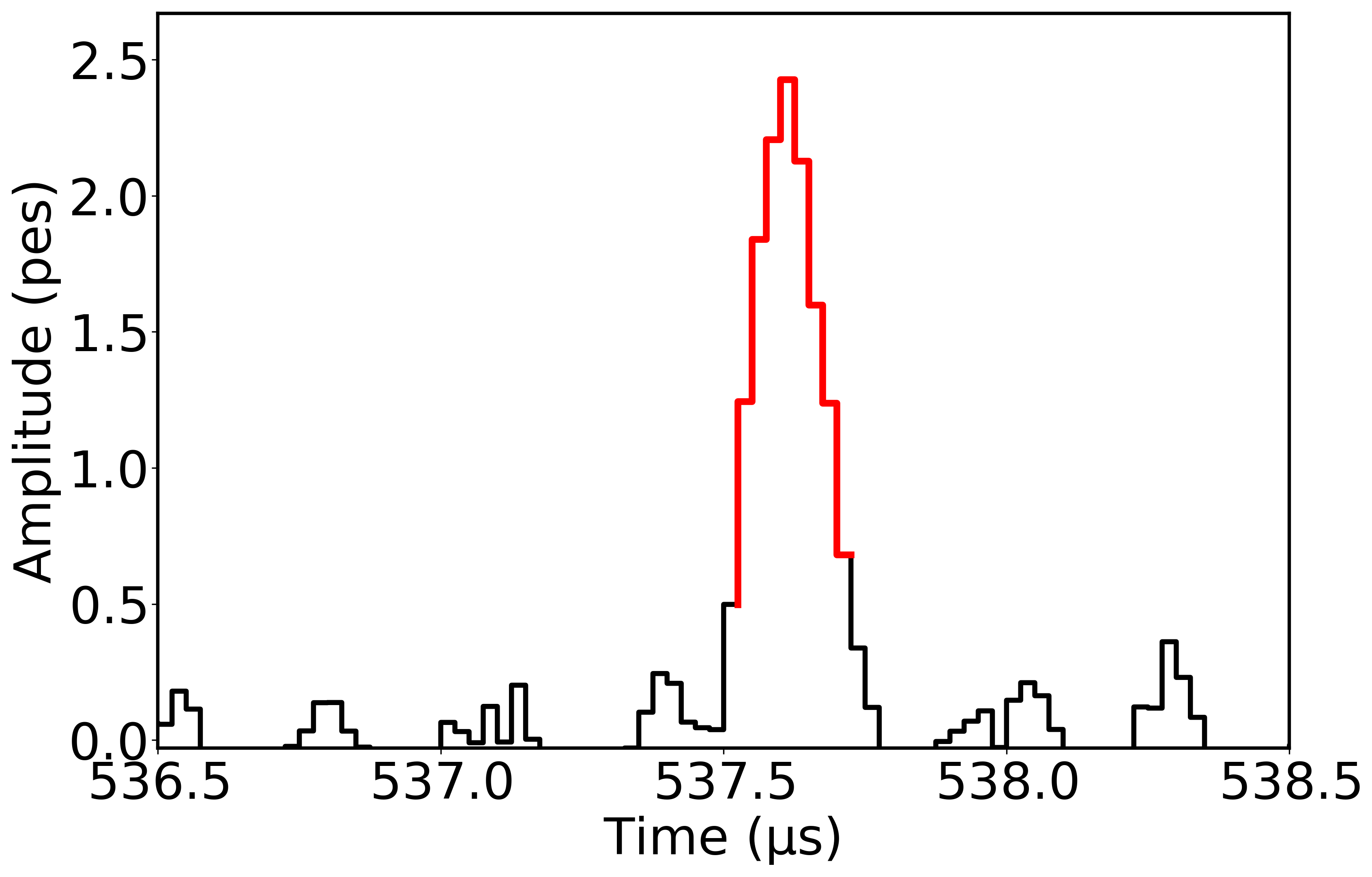
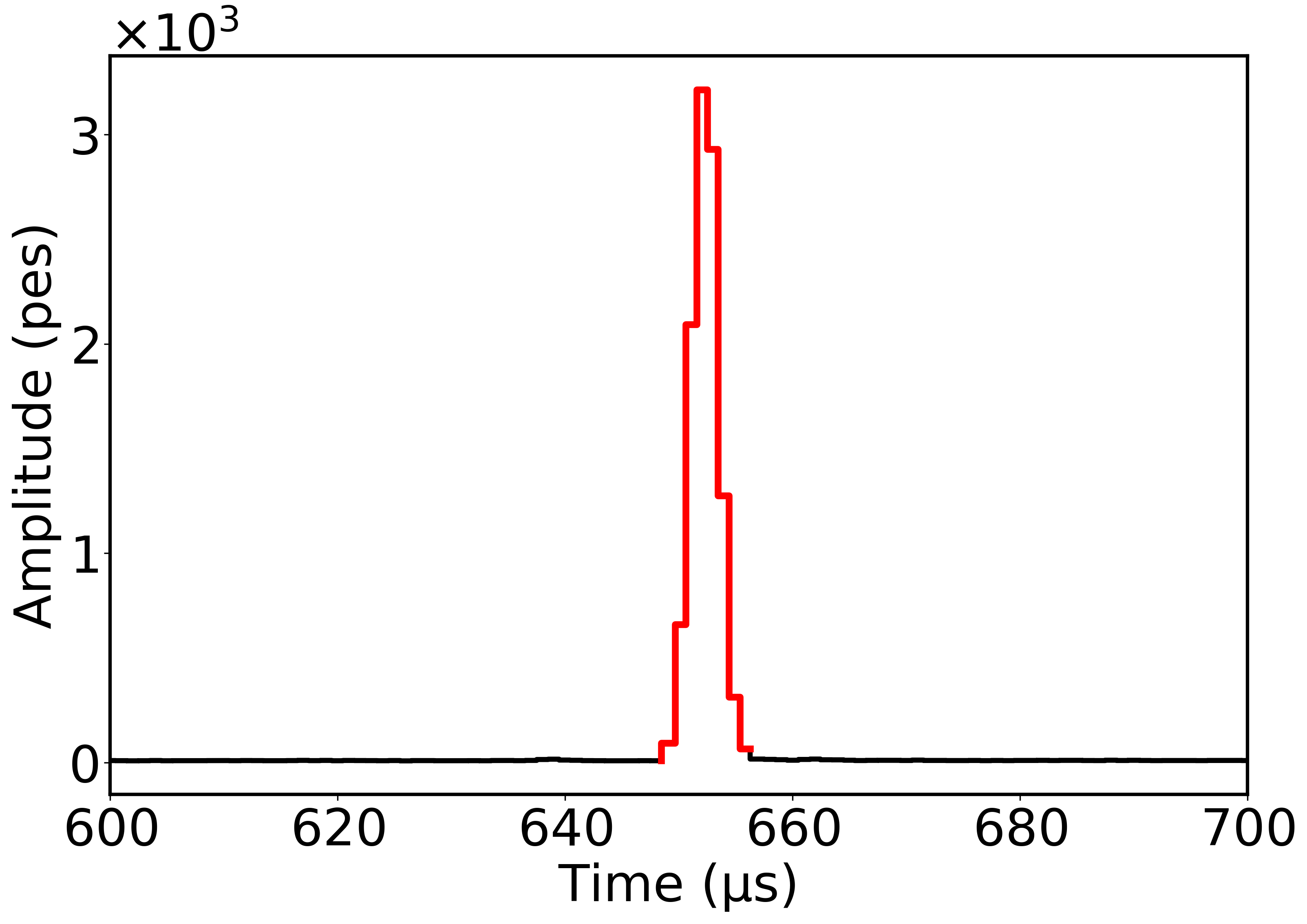
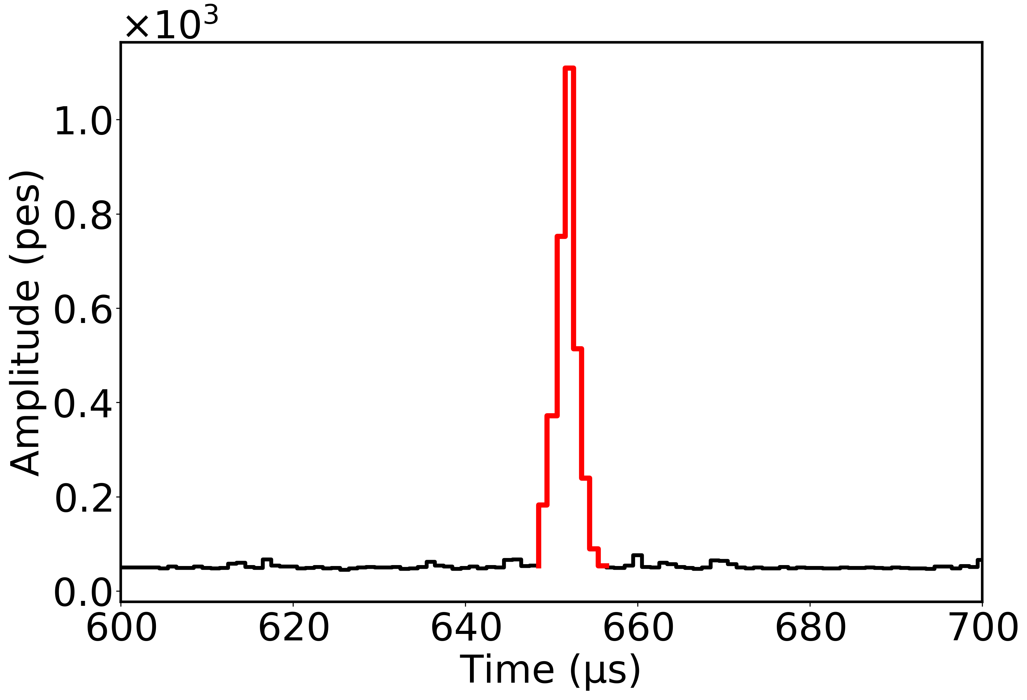
Finally all peaks are stored in a single PMap object. A PMap contains a list S1 peaks and a list of S2 peaks. Each Peak contains the times of the samples within the peak and a SensorResponse object for PMTs a SensorResponse object for SiPMs. Each SensorResponse object contains the IDs and the sliced waveforms of each sensor that contains signal in an event.
These data are stored in an hdf5 file in 5 separate tables under a common group PMAPS. See the output section for a full description.